Training SWE agents with Miles on MI355X: taming long‑tail trajectories and complex sandbox coordination
On this page
- TL;DR
- Background
- Why agentic RL is different
- Architecture
- The stack
- Experimental setup
- Where the time goes
- Step time breakdown
- The long-tail problem
- Context growth and the KV cache
- The CPU side: sandboxes
- The sandbox life cycle
- Cloud sandboxes at 384 concurrent trajectories
- What we learned
- Key fixes
- Results
- Solve rate
- Throughput
- Training stability
- Conclusion
- Next: frontier-scale agentic RL
- References
We trained Qwen3-30B-A3B-Instruct with fully asynchronous agentic RL on AMD Instinct MI355X using Miles, SGLang, Megatron-LM, and Harbor, nearly quadrupling its pass@1 score on a 100-task stratified subset of SWE-bench Verified, from 7.3% to 27.5%. The biggest bottlenecks were long-tail trajectories, CPU sandboxes, and data movement. We share how we addressed these challenges to improve throughput and accelerate learning, with lessons applicable to larger models such as DeepSeek-V4-Flash, GLM-5.3, and Kimi K3.
TL;DR
- SWE-bench Verified subset pass@1: 7.3% → 27.5%. Qwen3-30B-A3B-Instruct, evaluated on 100 stratified tasks with 4 attempts per task after SFT and agentic RL.
- ~4× rollout throughput: ~860 → ~3,480 trajectories/hour. The model and RL recipe stay fixed; inference scales from one to three 8-GPU MI355X nodes, with cloud sandboxes and concurrency fixes.
- ~3× faster RL steps: 850 s → 284 s. Capping trajectory length on the same 8-GPU inference node reduces the long tail.
- 384 concurrent agent sandboxes. The largest run uses three inference nodes and one training node, each with 8× MI355X.
Background
Why agentic RL is different
In coding agentic RL, one training sample is a whole episode. The model reads a GitHub issue, runs 20 to 100+ shell commands in a sandbox, edits code, and gets a reward only if the repository’s tests pass.
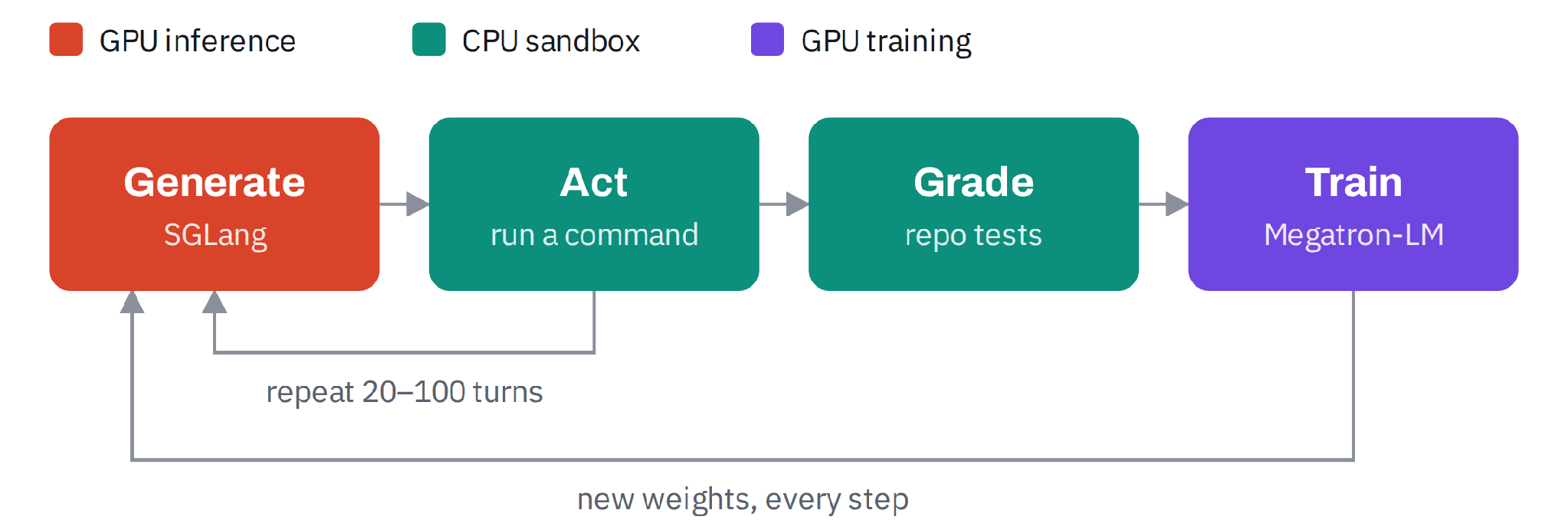
Figure 1: The agentic RL loop. One training sample is a whole multi-turn episode.
Compared with single-turn RL, this workload adds new problems:
-
Long-tail stragglers. Two attempts at the same task can differ 2.5× in length, and a GRPO group can’t be scored until its slowest attempt finishes, so a few stragglers can hold up training.
-
A CPU fleet on the critical path. Every trajectory needs its own sandbox for building and testing code.
Architecture
Inference and training run on separate nodes. The inference node runs eight single-GPU SGLang engines and Harbor, which manages the sandboxes. The training node runs Megatron-LM and pushes new weights back to the engines. Training is fully asynchronous, allowing rollout and training to overlap. The trainer proceeds once enough completed trajectories are available, rather than waiting for the slowest ones, reducing idle time and improving overall throughput.
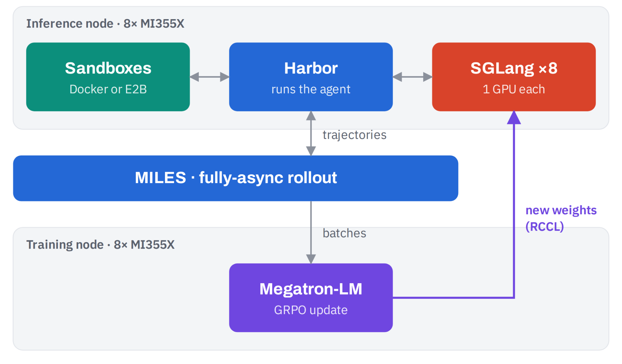
Figure 2: Architecture. Harbor runs each agent in a sandbox and calls the SGLang engines; Miles batches finished trajectories for Megatron, which sends new weights back.
The stack
Every layer is open source, and the whole system ships as one ROCm container.
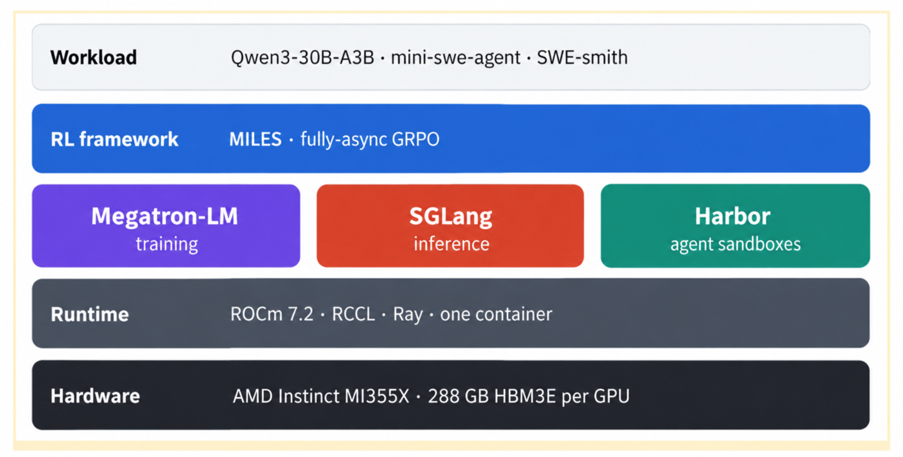
Figure 3: Software stack. Recipe: SFT on ~4,000 public agent traces (Open-SWE-Traces), then RL on ~1,350 SWE-smith tasks from 47 repositories that do not appear in SWE-bench Verified.
Experimental setup
We start from Qwen3-30B-A3B-Instruct and train it in two stages. SFT fine-tunes it for one epoch on about 4,000 successful agent traces from Open-SWE-Traces, which teaches the tool format. RL then runs fully asynchronous GRPO on about 1,350 SWE-smith tasks: 8 attempts per task, a reward of 1 when the repository’s tests pass, and no KL penalty. Each trajectory is limited to 8,192 generated tokens per turn, 65,536 tokens in total, and 80 turns.
| Item | Setting |
|---|---|
| Model | Qwen3-30B-A3B-Instruct |
| Hardware | AMD Instinct MI355X, 288 GB HBM3E per GPU; one inference node and one training node, 8 GPUs each (up to 4 nodes for the largest E2B run) |
| Software | Miles (fully asynchronous GRPO), SGLang, Megatron-LM, Harbor, ROCm 7.2, in one container |
| Agent | mini-swe-agent, one sandbox per trajectory (local Docker or E2B microVMs) |
| SFT data | ~4,000 public agent traces (Open-SWE-Traces) |
| RL data | ~1,350 SWE-smith tasks from 47 repositories that do not appear in SWE-bench Verified |
| Evaluation | SWE-bench Verified, 100-task stratified sample, 4 attempts per task, pass@1 |
Where the time goes
Step time breakdown
We profiled the training pipeline. Figure 4 shows the trainer-side step breakdown: actor updates account for 63% of the measured step, waiting for rollouts for 29%, and log-probability recomputation for 8%. Weight synchronization is logged separately. We also investigated rollout time, where LLM calls and waiting for CPU sandbox starts were the main bottlenecks.
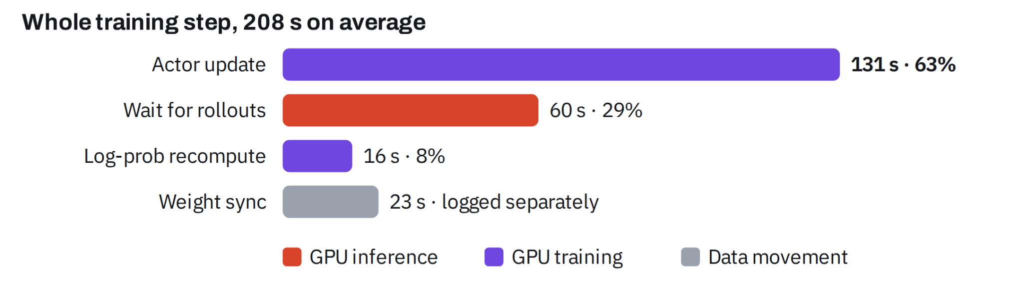
Figure 4: Trainer-side step breakdown in our 384-trajectory run (mean of 16 steps). The measured step averages 208 s; weight synchronization is logged separately. Limits: 8K generated tokens per turn, 64K tokens per trajectory, 80 turns.
The long-tail problem
In GRPO, every group waits for its slowest trajectory, and agents frequently run out of per-turn context: 84% of trajectories ran to the turn cap, while successful runs needed a median of only 8 turns. During the tail, engines decode a handful of sequences at a batch size near 1, so the GPUs sit mostly idle. 32% of the rollout time came after 90% of trajectories had finished.
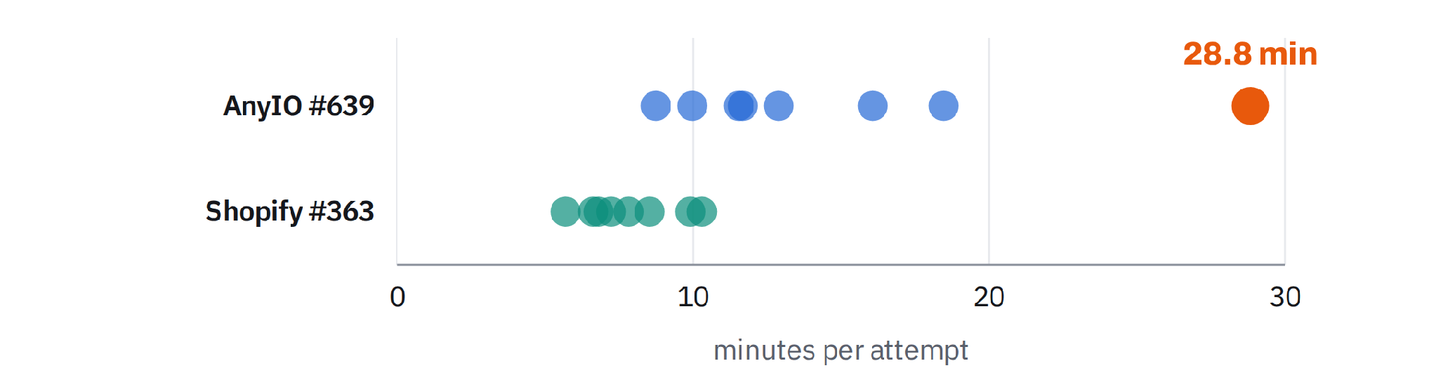
Figure 5: The long tail: 8 attempts at each of two tasks, same model, same batch. The slowest AnyIO attempt took 28.8 minutes.
We tried various tactics to mitigate this issue. Fully asynchronous training plus a tighter length cap gave us most of our speed-up: steps got 3× faster with no effect on successful runs.
Context growth and the KV cache
Each turn adds tool output to the context. At 96 KB per token, a 64K-token trajectory holds 6.3 GB of KV cache. In one run the engine had no context cap: a few generations grew to 113K–186K tokens, and about 10 of them filled the engine’s 1.5M-token KV cache. The other 99 requests queued on that engine got no tokens until they timed out. Capping context at 64K in the engine fixed this. With 288 GB of HBM, one MI355X engine holds tens of 64K-token trajectories at once.
The CPU side: sandboxes
The sandbox life cycle
Every trajectory needs its own clean environment with the repository, its dependencies and its tests. With hundreds in flight, sandboxes are a CPU fleet on the critical path: while an agent waits for one, its GPU slot does nothing.
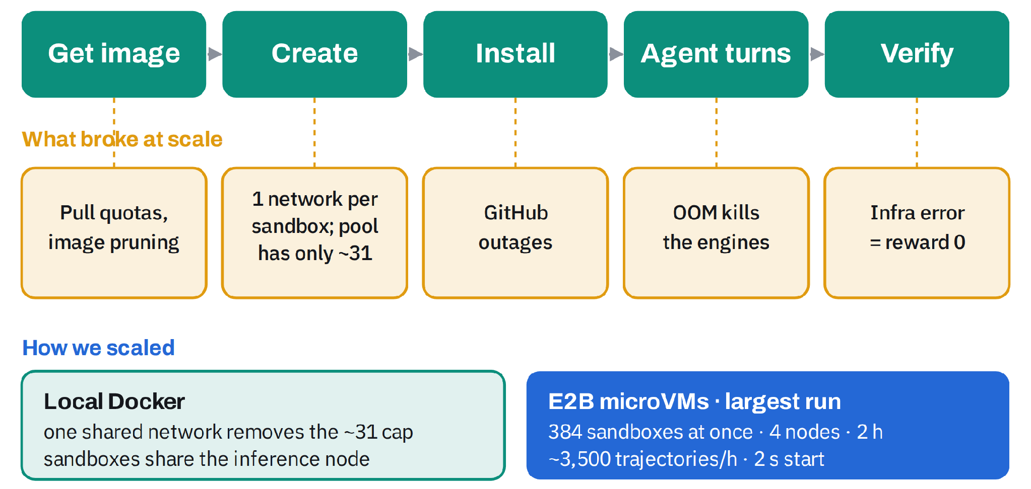
Figure 6: Each trajectory runs this sandbox life cycle on CPUs. Every stage failed in some way once we ran hundreds at once; the bottom row shows how far each sandbox option scaled.
Cloud sandboxes at 384 concurrent trajectories
To take sandboxes off the inference node, we moved them to E2B cloud microVMs (2 vCPUs and 4 GB each) and ran 384 trajectories (24 single-GPU SGLang engines at 16 trajectories each) at once across 4 nodes. After a mid-run restart, rollout throughput reached approximately 3,480 trajectories/hour, about 4× the local-Docker baseline.
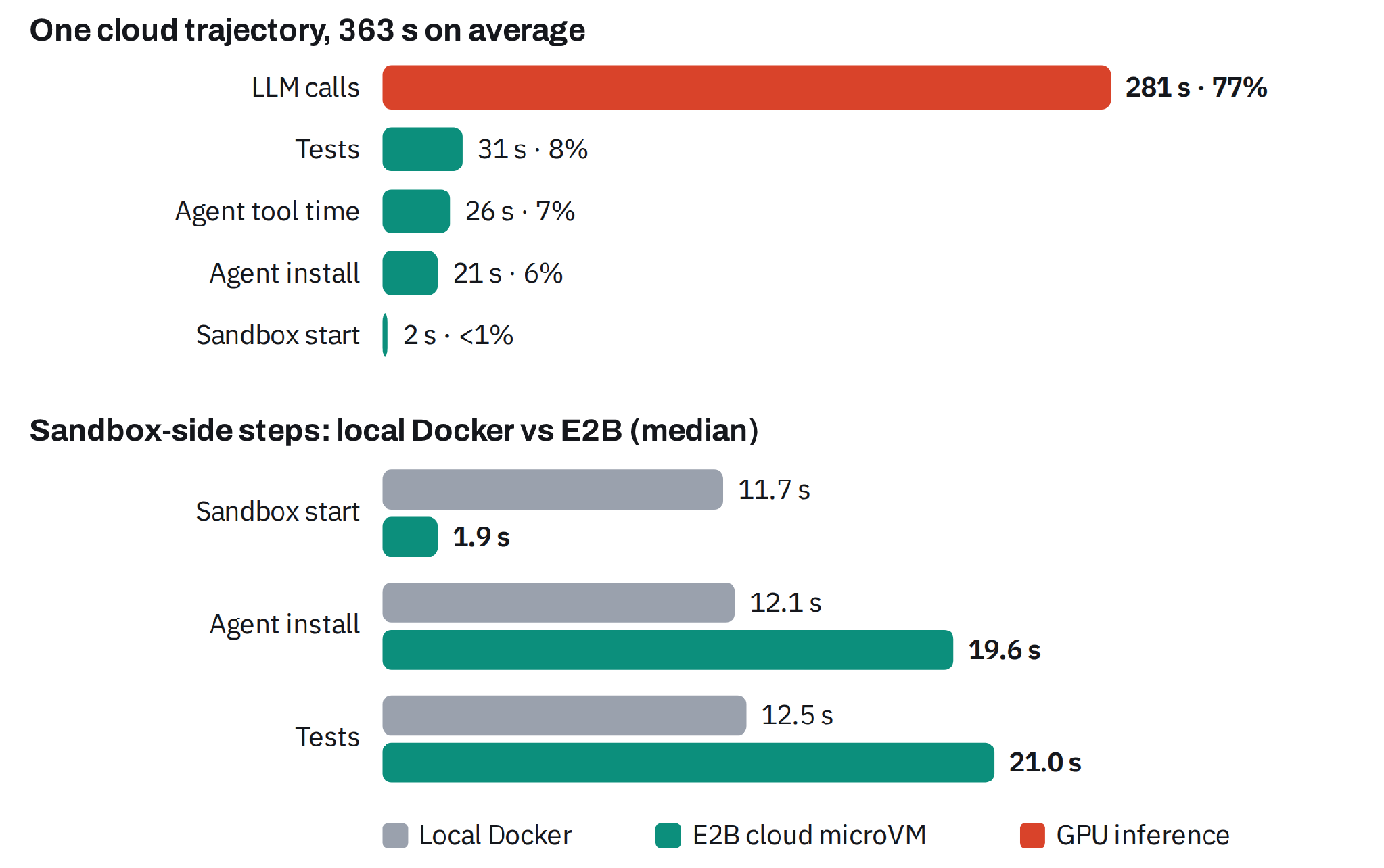
Figure 7: Top: where an E2B trajectory’s time goes at 384 concurrent trajectories (means over 4,211 trajectories that finished normally in steady state). Bottom: median time of the sandbox-side steps, local Docker vs E2B. Local Docker figures come from a 278-trajectory window of the same RL recipe.
-
Sandbox start stops being the cost. A cloud sandbox is ready in 1.9 s (median, 3.7 s at p99) and stays flat at 384, against 11.7 s for local Docker under load.
-
Steps that fetch or compute get slower. Installing the agent takes 7.5 s longer and running the tests 8.5 s longer in a 2-vCPU microVM, and each LLM call crosses a tunnel (about 0.26 s). A trajectory takes 15–40 s longer, 4–11% of its time.
-
The sandbox side is a fifth of the trajectory. LLM calls take 77% of a cloud trajectory; tests, tool calls, agent install and start together take 22%.
-
The GPUs had headroom. At 384 trajectories the engines had an empty queue and used at most 23% of the KV cache. The limit was sandbox concurrency, not GPUs.
-
Reliability held at scale. In steady state 2.6% of trajectories failed, and 0.09% of 300,500 tunnelled LLM calls returned an error.
What we learned
-
Start-up cost depends on the platform. On a self-hosted E2B that starts 3 sandboxes at a time, waiting for a start took 20% of trajectory time; E2B’s cloud service starts one in 1.9 s. The first call in a fresh sandbox was also 15× slower than a repeat call in microbenchmarks, so warm pools and snapshots matter more than extra cores.
-
Infrastructure failures become wrong rewards. 3.1% of trajectories ended in an infrastructure error, which scores 0 just like a wrong fix. The policy gets penalized for the infrastructure, so these failures must be logged and filtered.
-
Hidden limits break first, not the network. As we added agents, every failure came from a fixed cap: at most 31 Docker networks per machine, 100 image downloads per hour for the whole cluster, 100 agent connections in Miles, and one CPU core handling all agent requests. Removing these caps, not adding bandwidth, is what lets us scale.
Key fixes
Almost every problem looked like a GPU issue at first. Almost none were.
| Fix | Problem | Effect |
|---|---|---|
| Cap trajectory length | Before the length cap, failing agents could loop for 200+ turns and hold up the step | 3× faster steps |
| Remove hidden concurrency caps | An HTTP pool capped agents at 100; one proxy process serialized all LLM calls | Contributed to the ~4× rollout gain alongside inference scale-out and cloud sandboxes |
| One shared sandbox network | Docker allowed only ~31 sandbox networks per node | Hundreds of sandboxes per node |
| Cap context in the engine | Runaway generations filled the KV cache | No more KV thrashing |
| Pin the NCCL interface | Cross-node weight sync picked a duplicate Docker IP and hung | Reliable sync |
| Keep HIP graphs on, add a watchdog | Rare GPU faults; disabling graphs halved throughput | Full speed, auto-resume |
Results
Solve rate
Figure 8 tracks SWE-bench Verified pass@1 through each stage of the recipe, on a 100-task stratified subset of the 500 Verified tasks with 4 attempts per task. The base model solves 7.3% of tasks, and SFT on ~4,000 public agent traces lifts it to 12.8%. Agentic RL then adds another 14.7 points, reaching 27.5%: it more than doubles the SFT score and accounts for nearly three quarters of the total gain. All RL tasks come from SWE-smith repositories that do not appear in SWE-bench Verified, so this gain is measured on codebases the policy never saw during RL.
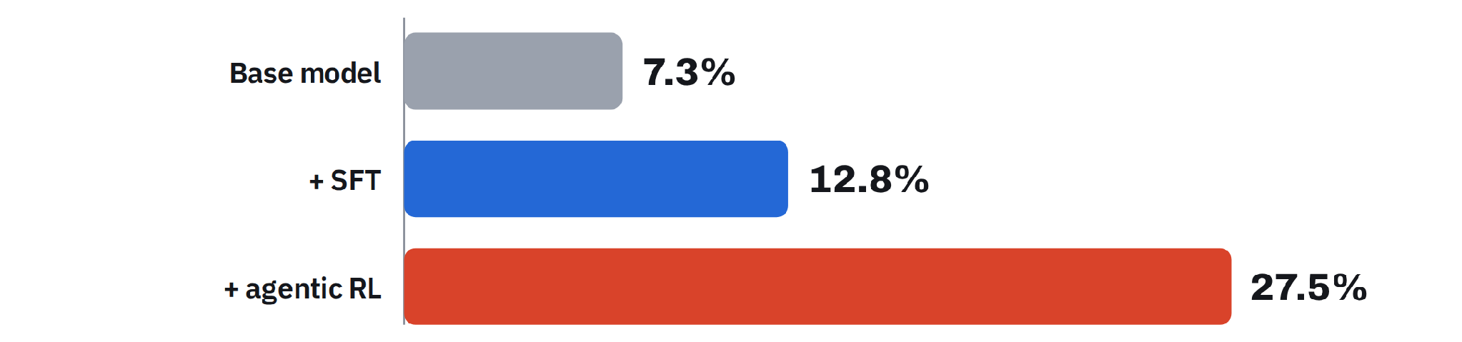
Figure 8: SWE-bench Verified solve rate (pass@1, 100-task stratified sample, 4 attempts each): 7.3% for the base model, 12.8% after SFT, and 27.5% after agentic RL.
Throughput
| Metric | Before | After |
|---|---|---|
| Training step time | 850 s | 284 s |
| Rollout throughput | ~860 trajectories/h | ~3,480 trajectories/h |
| Concurrent trajectories | ~100 | 384 |
| LLM call latency under load | 12.6 s | 4.4 s |
These measurements come from runs on two to four MI355X nodes, with the model and RL recipe held fixed. The ~4× rollout throughput gain combines inference scale-out from one to three 8-GPU nodes, cloud sandboxes, and removal of concurrency limits. The ~3× step-time gain comes from capping trajectory length on the same 8-GPU inference node. These are separate comparisons, rather than one fixed-hardware before/after run.
Training stability
The run trained for 145 steps and survived three restarts from checkpoint. Nothing in the curves drifts or blows up.
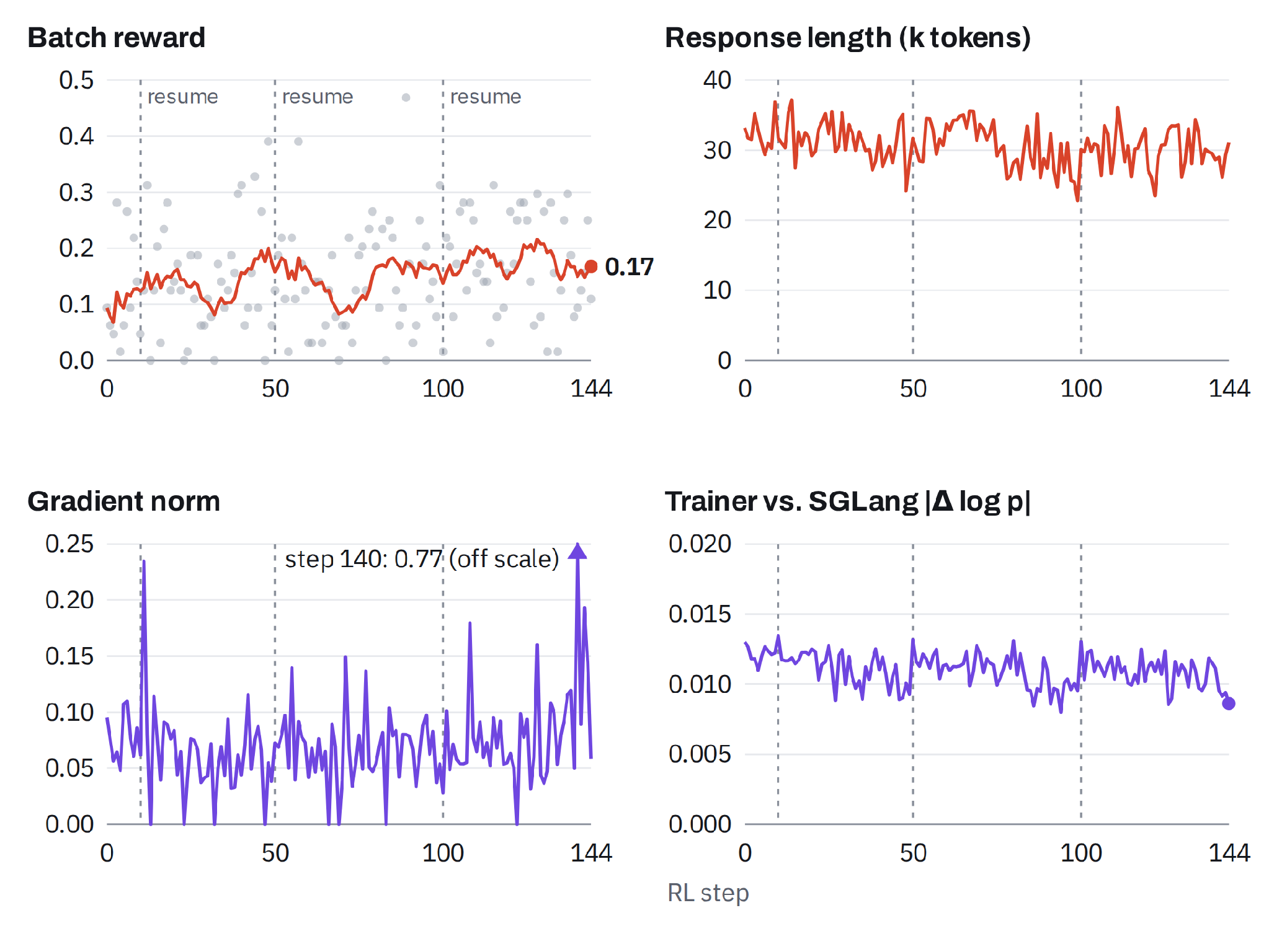
Figure 9: Training curves of the RL run behind the 27.5% result. Red is measured on rollouts, purple on the trainer. Grey dots are per-batch rewards (8 tasks × 8 attempts) and the line is a 10-step mean. Dashed lines mark resumes from the checkpoint. The gradient-norm axis is zoomed to its normal range, so the single off-scale step is drawn as a marker.
-
Reward climbs slowly and steadily. The 10-step mean rises from 0.13 to 0.17 on training tasks. Single batches swing between 0 and 0.47 because each batch draws new tasks.
-
Updates stay small. The median gradient norm is 0.07. One step (140) reached 0.77, still below the clipping threshold of 1.0, with no change in the trainer–inference gap or effective sample size. The next step was back at 0.09. Eight batches gave a zero gradient because no task in them had a mix of passing and failing attempts.
-
Trainer and inference engine agree. The mean per-token log-probability gap stays near 0.011 and falls slightly over the run. The effective sample size of the importance weights averages 93%, so off-policy correction rarely has to step in.
-
No length drift. Responses hold at about 30K tokens per trajectory, with no collapse toward short answers or blow-up toward the context cap.
Conclusion
Agentic RL runs end to end on AMD Instinct MI355X: Qwen3-30B-A3B-Instruct improved from 7.3% to 27.5% pass@1 on a 100-task stratified subset of SWE-bench Verified with stable training. With the model and RL recipe held fixed, scaling inference from one to three nodes, using cloud sandboxes, and removing concurrency limits delivered ~4× higher rollout throughput. Separately, capping trajectory length on the same 8-GPU inference node made training steps ~3× faster.
Next: frontier-scale agentic RL
-
Larger frontier models: Run the same recipe on DeepSeek-V4-Flash, GLM-5.3, and other models already tested with Miles on MI350-series GPUs.
-
Scale: Go past 384 concurrent sandboxes and spread inference across more nodes.
-
Stop wasted rollouts: Teach the agent to submit instead of looping to the turn cap.
-
Additional features: Study the benefits of sticky sessions and hierarchical KV caching.
-
More applications: Extend the study to other agentic workloads.
References
-
Miles, RL framework (SGLang + Megatron-LM)
-
ROCm Support for Miles, LMSYS blog
-
Harbor, agent and sandbox framework
-
mini-swe-agent · SWE-smith · Open-SWE-Traces · SWE-bench Verified