Pipeline Parallelism in SGLang: Scaling to Million-Token Contexts and Beyond

TL;DR

We are excited to introduce SGLang's highly optimized Pipeline Parallelism (PP) implementation, specifically engineered to tackle the challenges of ultra-long context inference. By integrating Chunked Pipeline Parallelism, Asynchronous P2P Communication, and a simple yet effective Dynamic Chunking mechanism, this PP design achieves industry-leading performance while ensuring seamless compatibility with other parallel strategies, PD Disaggregation, and HiCache. In multi-node deployments, scaling to PP4 TP8 with this implementation yields a 3.31× Prefill Throughput for DeepSeek-V3.1 on an H20 cluster compared to TP8 when the chunked prefill size is set to 12K, significantly outperforming the TP32 solution (2.54×) by a 30.5% margin. This highlights PP's inherent architectural advantage for large-scale, cross-node scaling over pure TP. Furthermore, our implementation also delivers up to a 67.9% reduction in TTFT while maintaining an 82.8% strong scaling efficiency, providing a highly efficient, open-source path for scaling trillion-parameter models for ultra-long context.

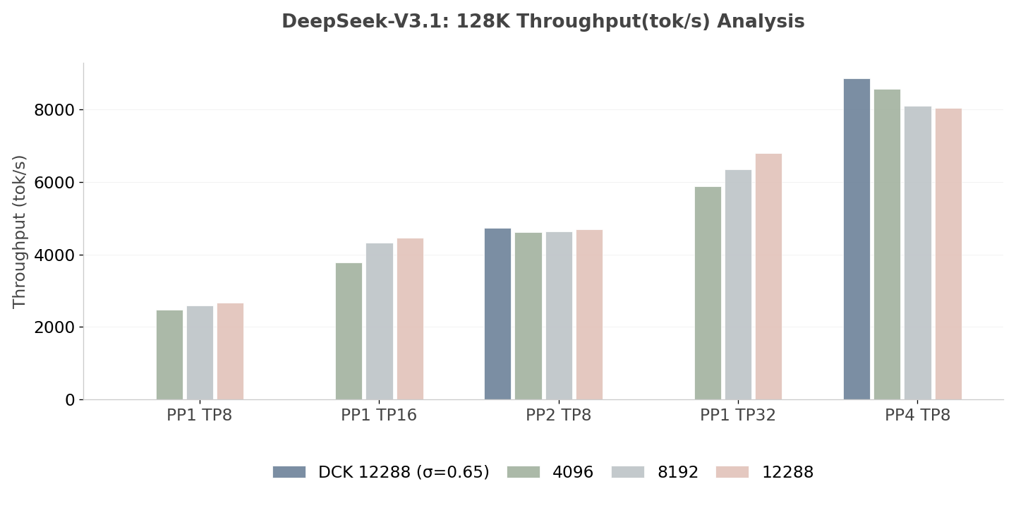
Prefill Throughput (Batch Size = 1) of DeepSeek-V3.1 on H20 (Higher is better)
Note: DCK 12288 (σ=0.65) means enabling Dynamic Chunking with the initial chunked prefill size set to 12K, and the smooth factor set to 0.65.

Introduction

As Large Language Models (LLMs) scale toward trillion-parameter architectures and "infinite" context windows, the underlying serving infrastructure must evolve toward more granular, cross-node parallelization strategies. While KV cache techniques effectively mitigate redundant computation, they cannot circumvent the prohibitive Time to First Token (TTFT) inherent in ultra-long sequences with extremely large initial Input Token Length (ITL). Although Tensor Parallelism (TP) remains the conventional approach for intra-node scaling, it frequently encounters communication bottlenecks during multi-node deployments. On the other hand, despite traditional Pipeline Parallelism (PP) addressing this bottleneck by reducing the communication volume, it struggles with resource underutilization and bubble overhead when processing such massive prompts.

Drawing inspiration from both open-source innovations and academic research, SGLang introduces a highly optimized Pipeline Parallelism implementation featuring Asynchronous Communication and Dynamic Chunked Prefill, which effectively minimizes the pipeline bubbles. By integrating these techniques, SGLang explores and reframes the processing of ultra-long prompts—effectively scaling away the prohibitive latency of long-sequence prefilling and transforming it into a high-throughput, computationally scalable streaming workflow.

Empirical benchmarks demonstrate that SGLang’s PP implementation achieves industry-leading performance. In large-scale deployments, it maintains over 80% scaling efficiency for various model architectures while scaling out to PP4, and it also delivers up to an 81% reduction in TTFT for ultra-long prompts when deploying Qwen3-235B-A22B-FP8 on H20 with PP8.

Background: Why Pipeline Parallelism?

To validate the necessity of Pipeline Parallelism (PP) for long-context prefill, it is essential to evaluate it against existing paradigms—specifically Tensor Parallelism (TP) and Context Parallelism (CP). While TP and CP offer distinct advantages, a theoretical and empirical decomposition of their communication volumes, bubble ratios, and implementation complexities reveals that PP occupies a unique, optimal position for multi-node scaling. The following analysis outlines the specific trade-offs inherent to each method.

1. Communication Volume and Scalability Analysis

The primary bottleneck in distributed inference scaling is inter-device communication. As model depth and sequence length increase, the volume of data transmitted between devices becomes a limiting factor, especially while scaling to large-scale and multi-node deployments.

Assuming $B$ stands for the Batch Size (often 1 for ultra-long context inference), $S$ for the total Sequence Length, $H$ for the Hidden State dimension, $L$ for the total Layer Number, $M$ for the Micro-batches size, and the activation precision is FP8 (1 byte). Based on this, we analyzed the communication volume of different parallel strategies.

• TP: TP splits individual weight tensors across multiple devices within a single layer. Due to this, TP incurs high communication overhead due to the necessity of synchronization after both the Attention Block and MLP Block. Consequently, the communication volume scales linearly with the number of layers. This frequent All-Reduce synchronization makes TP bandwidth-bound, limiting its scalability across large clusters. $$\text{Commu Volume}({TP}) = 2 \cdot (TP_{Size} - 1) \cdot \left( B \cdot S \cdot \frac{H}{TP_{Size}} \right) \cdot 2 \cdot L \cdot \text{bytes} \approx 4 \cdot B \cdot S \cdot H \cdot L \cdot \text{bytes}$$ (Note: Each All-Reduce involves $2 \times$ the data size in a ring-based implementation. Each layer involves $2 \times$ All-Reduce operations, one after the Attention Block, and one after the MLP Block.)
• CP: Similarly, CP requires extensive synchronization communication to aggregate Key-Value (KV) states across devices. Typically, CP utilizes All-Gather at every layer, resulting in significant latency penalties in bandwidth-constrained environments. $$\text{Commu Volume}({CP}) = (CP_{Size} - 1) \cdot \left( B \cdot \frac{S}{CP_{Size}} \cdot 2 \cdot H_{KV} \right) \cdot L \cdot \text{bytes} \approx 2 \cdot B \cdot S \cdot H_{KV} \cdot L \cdot \text{bytes}$$ (Note: Assuming CP utilizes Ring-Attention-based solution. For models utilizing GQA, $H_{KV}$ is smaller than $H$, which reduces CP's communication volume.)
• PP: In contrast, PP exhibits a significantly reduced communication footprint. Data is transferred only at the boundaries of pipeline stages, using Point-to-Point (P2P) primitives rather than collective operations. Since a stage typically contains multiple layers, the communication frequency is determined by the number of stages ($P$), not the total number of layers ($L$). Crucially, for a fixed model, as we increase the number of layers per stage, the communication volume remains constant at the boundaries. $$\text{Commu Volume}({PP}) = M \cdot \left( \frac{B}{M} \cdot S \cdot H \right) \cdot (P-1) \cdot \text{bytes} = B \cdot S \cdot H \cdot (P-1) \cdot \text{bytes}$$ (Note: In multi-node deployments where $P \ll L$, PP achieves a nearly order-of-magnitude reduction in total communication volume compared to TP.)

2. The Bubble Ratio Trade-off

While PP optimizes communication, it introduces pipeline bubbles—idle periods where devices wait for data dependencies. This presents a trade-off between communication efficiency and device utilization.

• TP and CP: Both methods achieve a zero bubble ratio theoretically, as all devices compute simultaneously on different parts of the same tensor or sequence. This maximizes compute intensity, assuming communication does not stall computation.
• PP: PP inevitably incurs a bubble ratio, quantified by the interaction between the PP Size ($P$) and the number of Micro-batches ($M$): $$ \text{Bubble Ratio} = \frac{P - 1}{P - 1 + M} $$ However, for long-context prefill scenarios where the workload is substantial ($M \gg P$), this ratio decreases significantly, rendering the efficiency loss negligible compared to the communication gains. In the Performance Impact section, we will evaluate the Strong Scaling Efficiency (i.e., the number of processors is increased while the problem size remains constant) of our PP implementation.

It is worth noting that while PP offers a distinct advantage in cross-node scaling, where communication bandwidth often becomes the primary bottleneck, a pure high-degree PP configuration is generally not recommended. This is because, for a fixed workload $M$, the pipeline bubble ratio increases proportionally with the PP size $P$. Instead, a better strategy is to leverage bubble-free parallel methods, such as TP or CP, for intra-node scaling. Since intra-node communication typically utilizes high-bandwidth interconnects like NVLink, these collectives are far less likely to become a performance bottleneck compared to cross-node transfers, allowing the system to maximize compute utilization without incurring additional pipeline overhead.

3. Implementation Complexity and Architectural Generality

The implementation complexity and architectural generality of a new feature are critical factors for a modern inference system, especially for an open-source project.

• TP: TP is easy to implement and widely supported. However, large-scale TP configurations are inherently inapplicable, as the granularity required for the quantization block sometimes cannot be aligned with the partitioning constraints imposed by MoE FFN weights. Consequently, even disregarding communication volume and overhead, larger TP is often precluded in multi-node scaling scenarios due to this incompatibility with quantization, which is a critical and indispensable optimization technique.
• CP: CP is complex, which requires specific, often intrusive modifications to the attention mechanism (e.g., Ring Attention). These changes must be tailored for every attention variant and specific model, reducing generality.
• PP: PP represents a medium complexity. It requires partitioning the model but remains agnostic to the internal mechanics of the layers. This makes PP a general-purpose solution applicable to all model architectures without requiring kernel-level rewrites for specific attention variants. To some extent, eliminating PP bubbles is more difficult than implementing PP itself.

Metric	Tensor Parallelism (TP)	Context Parallelism (CP)	Pipeline Parallelism (PP)
Split Dimension	Hidden State ($H$)	Sequence ($S$)	Layer ($L$)
Communication Pattern	AllReduce (Per Layer)	AllGather (Per Layer)	P2P (Send/Recv)
Communication Volume	High	Medium	Low
Bubble Ratio	0	0	$\frac{P - 1}{P - 1 + M}$
Implementation Complexity	Low	High (Attention-variant specific)	Medium
Architectural Generality	High	Low	High

In conclusion, the balance of the generality and scaling efficiency makes PP not merely an alternative, but a necessary component for scaling long-context prefill to massive, multi-node clusters where TP and CP encounter bandwidth ceilings. In the meantime, CP has the potential to complement TP for intra-node bubble-free scaling and acceleration. PP × CP is already under development (Future Roadmap), which will be included in Part II of this blog.

The Challenge: The "Bubble" and The "Wall"

In a traditional Pipeline Parallelism setup, the model layers are partitioned across GPUs (Stage 1 to Stage N). When serving standard requests (e.g., < 4K tokens), it normally works well. However, when processing a prompt exceeding 128K or even 1M tokens, two critical issues emerge:

1. The Pipeline Bubble: Processing prompts as monolithic batches forces downstream GPUs into prolonged idle states, creating massive 'pipeline bubbles' that severely degrade throughput.
2. The Memory Wall: Processing a 1-million-token prompt in a single pass requires storing and communicating intermediate hidden states for the entire sequence, resulting in significant overhead and peak memory footprint.

The SGLang Pipeline Parallelism Architecture

SGLang’s pipeline implementation goes beyond the standard "sequential" approach. We’ve introduced several advanced features to minimize "bubbles" (i.e., GPU idle time) and maximize hardware utilization.

1. Chunked Pipeline Parallelism (CPP)

Processing a 1-million-token prompt in a single forward pass would lead to massive bubbles as later stages wait for the first stage to finish. Inspired by architectures like Mooncake[1], BladeLLM[2], and TeraPipe[3], SGLang supports Chunked Pipeline Parallelism. Instead of feeding the full prompt into the pipeline, SGLang partitions the prompt into smaller "chunks" (e.g., 4K or 6K tokens). These chunks flow through the pipeline stages like micro-batches. By breaking long prompts into smaller chunks, the system can "pipeline" the prefill phase. As soon as the first stage finishes computing the hidden states for Chunk 1 and initiates PP communication, it immediately moves to processing Chunk 2, while Stage 2 simultaneously begins processing Chunk 1. This reduces the pipeline startup latency from being proportional to the total sequence length to being proportional only to the first chunk size.

This approach marks a critical first step from an engineering perspective to tackle the challenges of ultra-long contexts. Notably, SGLang pioneered the support for this feature more than six months ago (#5724, #8846), underscoring its long-standing commitment to optimizing real-world, long-context inference.

2. Better Overlapping: Micro-batching and Async P2P Communication

Although combining Pipeline Parallelism and Chunked Prefill can significantly reduce communication volume compared to tensor parallelism, it often suffers from pipeline bubbles where the GPU blocks while waiting for CPU metadata processing or network transfers. To eliminate this performance hazard, SGLang implements a Micro-batching Event Loop with non-blocking asynchronous peer-to-peer (P2P) communication to overlap GPU computation with CPU metadata processing and PP communication. This ensures that while one micro-batch is being computed on the GPU, the next one is already being prepared and moved into position effectively, ensuring the pipeline remains as saturated as possible. The code is available here.

The key mechanisms of the implementation include:

• Decoupled Sync/Async Logic in the Event Loop: The scheduler uses async_send in _pp_send_pyobj_to_next_stage. Instead of waiting for a transfer to complete, it returns a P2PWork handle. The actual synchronization (P2PWork.work.wait()) is deferred until _pp_commit_comm_work is called, allowing the CPU to perform other work—like scheduling the next batch or processing metadata—while data is in flight.
• Multi-Stream Execution: In addition to the main default_stream, which serves as the synchronization stream, SGLang utilizes dedicated forward_stream and copy_stream to execute forward pass GPU computation and Data-to-Host (D2H) memory transfers separately for better overlapping. While _pp_launch_batch is executing the current micro-batch on the GPU for the current stage, the CPU processes the previous micro-batch's results using _pp_process_batch_result.

3. Advanced Option: Dynamic chunking

With Chunked Pipeline Parallelism and Async P2P communication, SGLang already achieves over 80% strong scaling efficiency as the PP size increases to 4. However, Chunked prefill with a fixed size can still cause bubbles in the pipeline, and this inefficiency becomes more pronounced as the PP degree increases. The main reason behind this phenomenon is that the model exhibits non-uniform execution latency across chunks of identical size, primarily due to the incremental nature of self-attention. As the prefix sequence length grows, the per-chunk processing time increases non-linearly. These timing mismatches propagate through the pipeline, compounding efficiency losses at higher PP ranks.

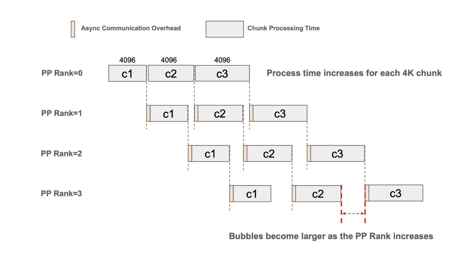
Fig. 1: Pipeline diagram with fixed chunked prefill size

We tested different models using a large PP size and found that they all conformed to this conclusion. Below is the profile result of a typical case.

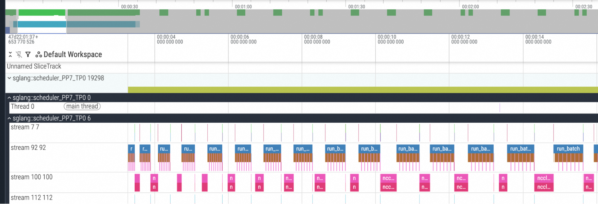
Fig. 2: Profile result of the PP rank 7 with fixed chunked prefill size

Therefore, if SGLang still utilizes a fixed chunked prefill size for CPP, the pipeline bubble ratio will be greater than the theoretical expectation (i.e., $\frac{P - 1}{P - 1 + M}$).

To address this issue, SGLang introduces a dynamic chunking mechanism to predict the optimal size for the next chunk such that it satisfies this condition:

$$ \text{Runtime}(L + \Delta L) - \text{Runtime}(L) = \text{Runtime}(\text{Initial Chunk Size}) $$

where $L$ denotes the Prefix Sequence Length, and $\Delta L$ denotes the Next Chunk Size. By profiling a series of requests with different ITLs, we model the cumulative runtime as a quadratic function of sequence length. Using this model, we solve the optimal next chunk size $\Delta L$ for any given prefix length $L$. Since the computation/communication complexity of the Attention mechanism scales with $L$, the next chunk size will be progressively reduced as $L$ grows to maintain an aligned chunk execution time across pipeline stages.

Based on this method, the scheduler can predict and dynamically reduce the chunk size during runtime to minimize the bubbles caused by the stage misalignment. To be noticed, the scheduler does not use the raw predicted value. To facilitate efficient KVCache memory management and ensure affinity with hardware execution efficiency, the value is aligned downward to the nearest multiple of max(--page-size, 64).

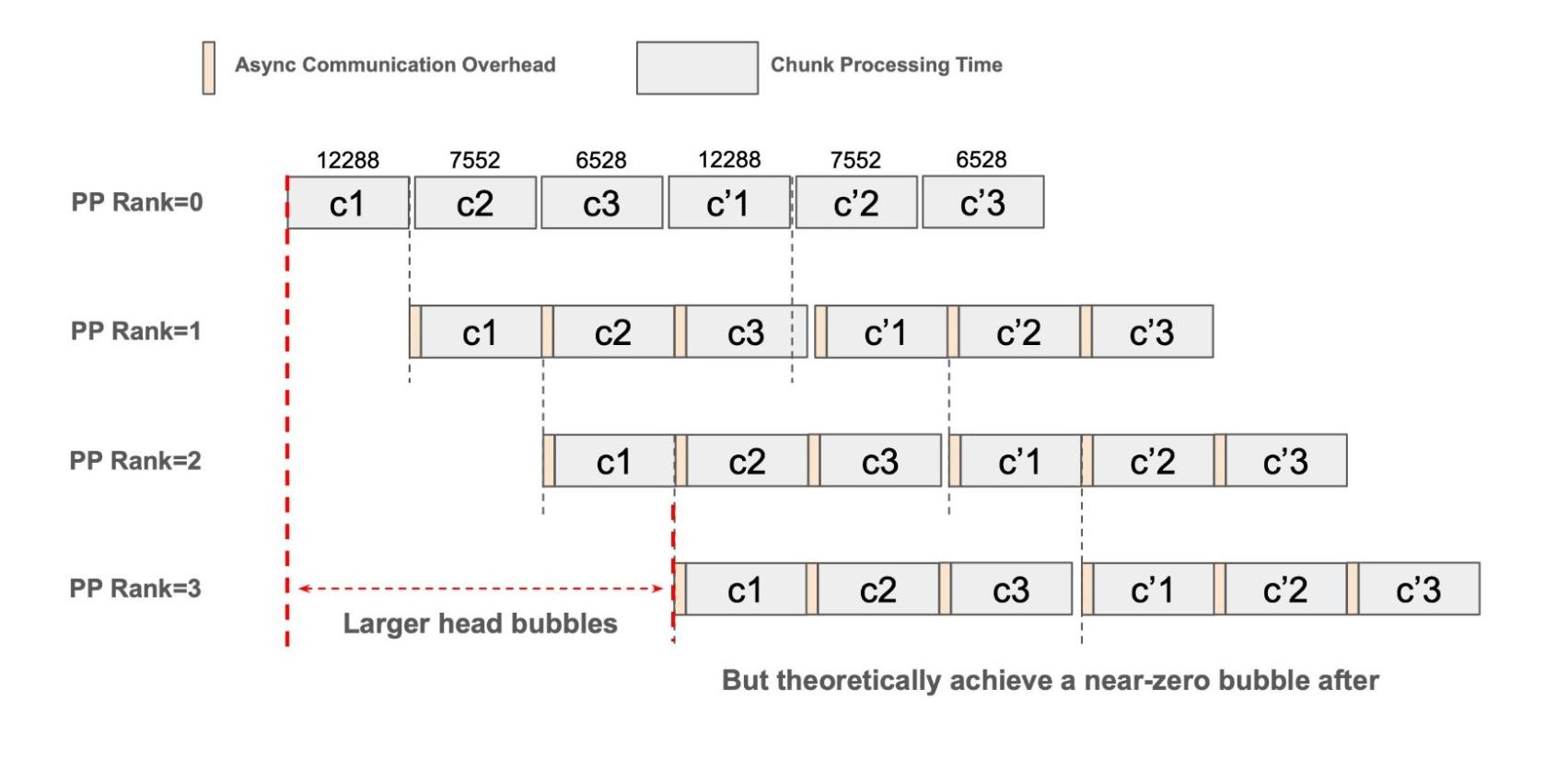
Fig. 3: Pipeline diagram with perfect dynamic chunking

However, due to the variation in hardware, models, and target workloads, a static configuration is seldom optimal across all scenarios. Consequently, achieving peak performance necessitates a degree of hyperparameter tuning when switching to the dynamic chunking mode. Also, we find that it is hard to perfectly fit the quadratic function due to the kernel performance variation of different shapes. Therefore, we introduce an environmental variable (SGLANG_DYNAMIC_CHUNKING_SMOOTH_FACTOR) to smooth the reduction for the dynamic chunking algorithm, defaulting to 0.75, which determines how much the chunk size can change during the prefill phase. A larger value leads to more aggressive chunk size reduction, potentially improving performance but increasing the total number of chunks (the chunk size at the end may become very small, which could lead to performance degradation).

Tuning Guidance for Dynamic Chunked Prefill

• Step 1 - Iterate to find the optimal fixed chunked prefill size for the targeted PP size: Different PP sizes for targeted ITL may have different optimal chunked prefill sizes. Therefore, users should iterate to obtain the baseline according to the available resources for scaling.
• Step 2 - Initial Chunk Size Selection for Dynamic Chunking: Set the initial size to 2× or 3× the optimal fixed chunked prefill size. This reduces the total number of chunks and prevents "tail chunks" from underutilizing hardware. To maintain efficiency for extremely large Input Token Lengths (ITL), the dynamic predictor automatically ensures subsequent chunks are at least 1/4 of this initial size. In addition, it is recommended to use a larger initial chunk size (e.g., 4× the optimal fixed chunked prefill size) for such cases as well.
• Step 3 - Smooth Factor Adjustment: This factor controls how strictly the chunk size adjusts the prediction given by the quadratic performance fitting model.
  • 1.0: Follows the model strictly.
  • 0.6 – 0.85 (Recommended): Typical range for the best balance between dynamic scaling and hardware stability. Through experiments, we find that a range between 0.6 and 0.85 typically yields the best performance for dynamic chunking, as depicted in Fig. 4 and Fig. 5.
  • 0: Disables dynamic adjustment, reverting to traditional fixed-size chunking.

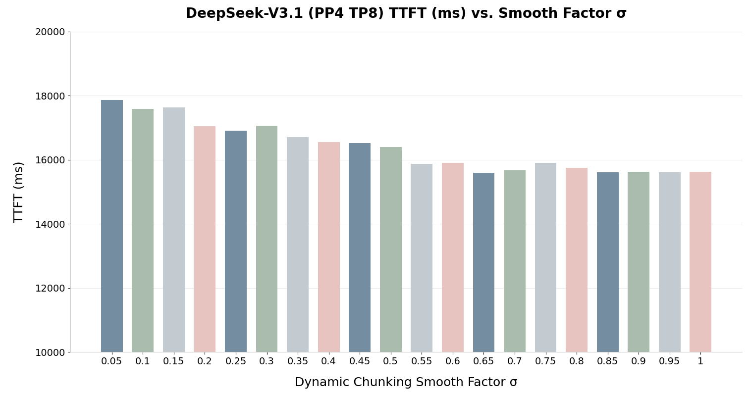
Fig. 4: Example of tuning the smooth factor for DeepSeek-V3.1 (Lower is better)

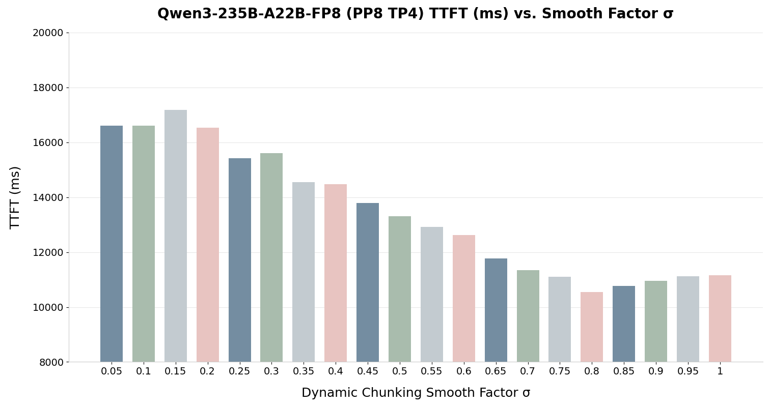
Fig. 5: Example of tuning the smooth factor for Qwen3-235B-A22B-FP8 (Lower is better)

• Another small optimization tip: Put the larger partition in the higher PP rank when the layers are not evenly divisible across ranks. It can increase the GPU utilization when a larger PP rank is waiting for the previous stage’s result, hence reducing the bubbles on higher PP ranks. If we take DeepSeek-V3.1 as an example, SGLANG_PP_LAYER_PARTITION=15,15,15,16 usually performs better than 16,15,15,15.

To validate the effectiveness of these combined strategies, we profiled the execution of DeepSeek-V3.1 using dynamic chunking. As observed in the following profile result of PP rank 3, the pipeline bubbles are significantly minimized compared to the static chunking approach, resulting in a more saturated execution.

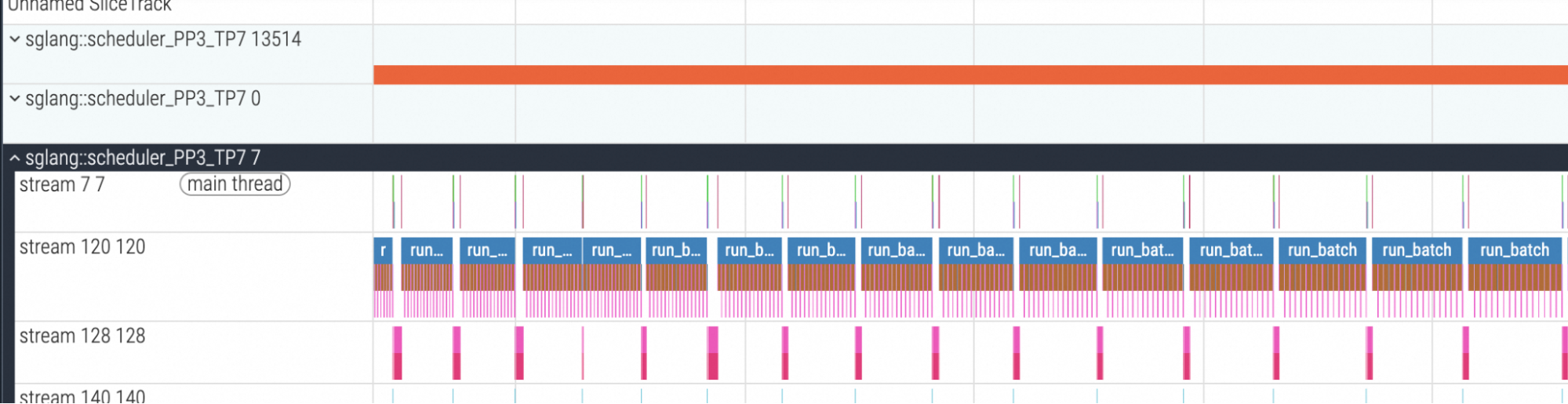
Fig. 6: Profile result of the PP rank 3 with dynamic chunking (DeepSeek-V3.1)

4. Production Ready: Compatibility with PD Disaggregation and HiCache

A unique strength of SGLang is its native support for Prefill-Decode (PD) Disaggregation within a pipelined setup. In a disaggregated cluster, the prefill nodes can use a high degree of PP to handle extremely long-context prompts, while the decode nodes can utilize a different parallelism strategy (like high-degree TP) to maximize token-generation speed.

• Chunk by Chunk KVCache Transfer: Instead of waiting for all chunks to be completed, SGLang supports transfer engine backends like mooncake, which can transfer the KVCache of one chunk from the prefill node to the decode node immediately when PD Disaggregation is enabled. This feature greatly reduces the KVCache transfer overhead.
• Flexible Hybrid Strategies: SGLang allows users to mix and utilize multiple parallelisms with PD Disaggregation. You can run PP8 TP8 for heavy prefill tasks on one set of nodes for prefill and apply other combinations, such as PP1 TP8, PP8 TP1, and PP1 DP16 EP16 for high-throughput decoding, optimizing for different phases of the inference lifecycle. This allows users to meet the expected Time To First Token (TTFT) and TPOT targets for production in a highly customizable way.
• Memory Efficiency: By distributing model weights across devices, PP reduces the per-GPU memory footprint, allowing for larger KV caches and higher concurrency. Therefore, it can be used to scale the max context length in some cases.

When handling contexts exceeding 128K tokens, SGLang also supports Chunked Pipeline Parallelism with HiCache, a distributed hierarchical KV cache system to further reduce the TTFT of multi-turn QA and agentic applications for ultra-long initial ITL:

• Semantic Prefix Matching: SGLang’s HiCache uses a radix-tree-based hierarchy to match prefixes at the chunk level. When a long-context request arrives, SGLang can perform a Hierarchical Cache Look-up. If the prefix tokens (processed in previous chunks) are already cached in the HiCache "Storage" layer (e.g., host memory or local disk), the PP pipeline can skip those chunks entirely, drastically reducing TTFT.

Performance Impact

This section provides a rigorous quantitative evaluation of the PP performance characteristics of the DeepSeek-V3.1 and Qwen3-235B-A22B-FP8 models. The analysis focuses on the interplay between PP size, Dynamic Chunking (DCK), and hardware scalability.

Our experimental testbed is a small cluster of 6 H20 nodes (8 × 96GB VRAM GPUs). Due to limited testing resources, experiments with a PP degree of 8 for DeepSeek-V3.1 were not conducted. Additionally, for the PP size = 1 configuration of DeepSeek-V3.1, we used a standalone H20 node (8 × 141GB VRAM GPUs) to obtain the baseline performance for an input token length of 128K (OOM will occur on the 96GB VRAM version). To better verify the throughput performance when the pipeline is saturated, we benchmarked and measured the average of 16 consecutive requests during the throughput test.

Note: We use the notation DCK to denote the chunked prefill size setup when enabling the dynamic chunking, and σ stands for the smooth factor of dynamic chunking. To conduct experiments with extremely long contexts, we overwrote the context length of the aforementioned model to 1 million, solely for performance analysis. Furthermore, we attempted to conduct experiments for DeepSeek-V3.1 with TP32 and Qwen3-235B-A22B-FP8 with TP8, but unfortunately, large TP configurations are inherently unsupported because the weight quantization block can not be divided by the FFN (MoE) layers' weight (Reference Issue). To thoroughly compare the differences between TP and PP in multi-node scaling scenarios, we hacked the model implementation file (skip parts of weight loading in load_weights) and config.json (Work Around Issue) of DeepSeek-V3.1, and managed to get TP32 runnable solely for performance verification purposes.

Input Token Throughput and Strong Scaling Efficiency

The analysis of Throughput vs. PP size demonstrates strong horizontal scalability across both model families, though the degree of scaling efficiency varies by configuration.

• PP vs. TP: A critical observation from the experimental data is the performance degradation observed when scaling Tensor Parallelism (TP) to 16, compared to a hybrid Parallelism approach (PP2 TP8). Despite utilizing an identical aggregate GPU count, PP2 TP8 consistently outperforms PP1 TP16 in both throughput and latency metrics. In addition, PP4 TP8 also consistently outperforms PP1 TP32 in both throughput and latency metrics for all chunk size configurations. Notably, under a fixed chunk size of 12288, this setup exhibits the lowest performance among all the chunking strategy setups for PP4 TP8. However, the worst performance of PP4 TP8 still surpasses PP1 TP32 (with a fixed chunk size also equal to 12288) by a significant margin of 18.4%, even though this setup already represents the best performance for tested pure TP configurations. And with dynamic chunking, this margin increases to 30.5%. Such results highlight the inherent advantage of the PP approach.
• Superior Scalability of DCK: The Qwen DCK 18K configuration exhibits the highest scalability, achieving a speedup factor of 6.14× for PP8 (32 GPUs) compared to PP1 (4 GPUs). This performance suggests that the dynamic adjustment of chunk sizes optimizes the balance between computational intensity and inter-node communication latency.
• Architectural Comparison: DeepSeek models demonstrate comparable scaling trajectories to Qwen up to the PP4 threshold. Notably, the DeepSeek DCK 12K (3.31×) marginally outperforms the static 4K variant (3.20×), validating the cross-architectural robustness of the Dynamic Chunking strategy in enhancing throughput.

Fig. 7: Throughput Analysis of DeepSeek-V3.1 (Higher is better)

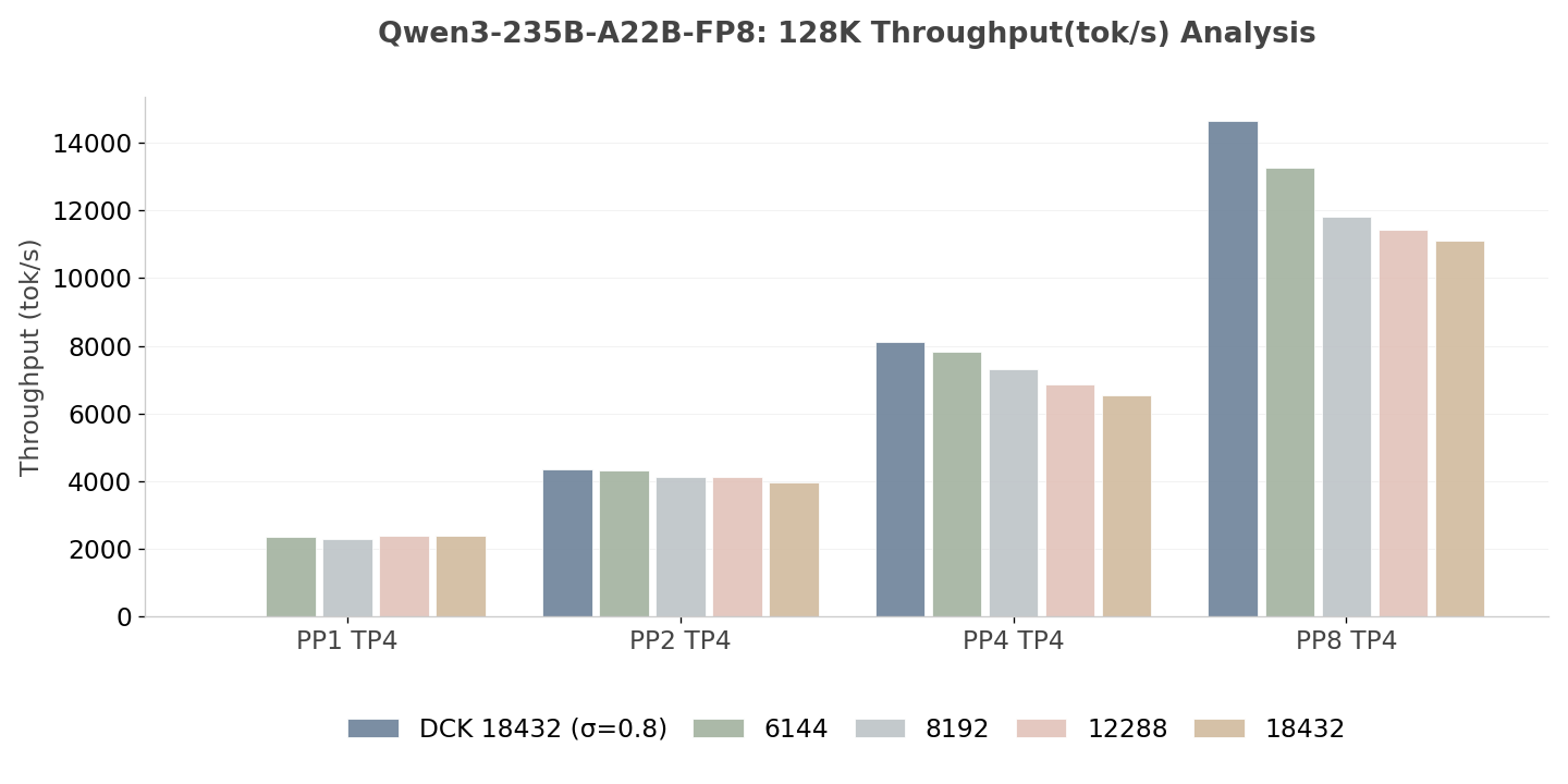
Fig. 8: Throughput Analysis of Qwen3-235B-A22B-FP8 (Higher is better)

The Strong Scaling Efficiency curves illustrate the degradation of hardware utilization as the system scales (for the strong scaling efficiency analysis, the ITL remains 128K while $P$ increases, thus the bubble ratio lower bound will definitely be higher according to the formula). All configurations exhibit a monotonic decay in efficiency as PP size (GPU counts) increases. However, Qwen DCK 18K still maintains a superior efficiency of 76.9% at the PP8 scale, whereas the static 6K configuration drops to 69.6%. This confirms that larger, dynamically managed chunks are more resilient to performance degradation caused by pipeline bubbles. Due to resource constraints, DeepSeek-V3.1 was evaluated up to PP size = 4, maintaining an efficiency of 82.8%. Extrapolating the current slope suggests that DeepSeek would likely follow a similar efficiency trajectory to Qwen, where DCK is projected to outperform the fixed chunking strategy.

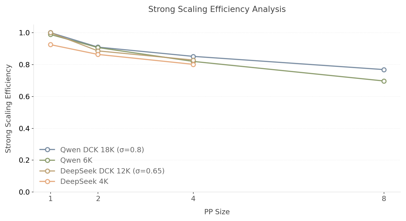
Fig. 9: Strong Scaling Efficiency vs. PP Size Analysis (Higher is better)

Reduced TTFT and Scaling Out for 1 million ITL

From Fig.10 and Fig. 11, we can observe that increasing the PP size from PP1 to PP4 can yield a substantial reduction in TTFT for both the fixed chunked setting and dynamic chunking. But dynamic chunking performs better for different PP setups. For the Qwen3-235B-A22B-FP8, the baseline TTFT of ~55.5s (PP1 TP4) is reduced to ~10.5s under the PP8 TP4 configuration, representing a latency improvement of approximately 81.1%. And for the DeepSeek-V3.1, the baseline TTFT of ~48.5s (PP1 TP8) is reduced to ~15.5s under the PP4 TP8 configuration, depicting a latency improvement of approximately 67.9%. These results indicate that Chunked Pipeline Parallelism is highly effective for reducing TTFT.

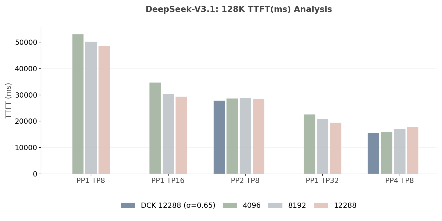
Fig. 10: TTFT Analysis of DeepSeek-V3.1 (Lower is better)

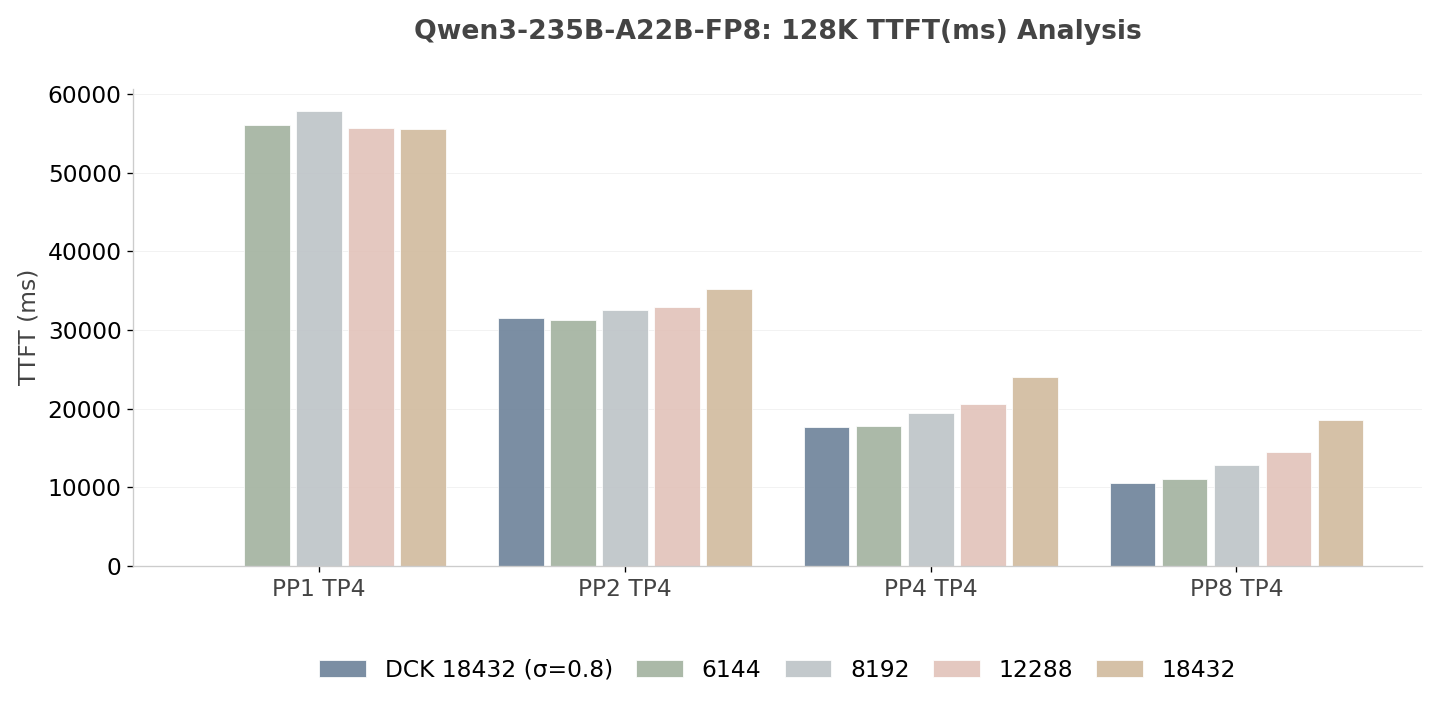
Fig. 11: TTFT Analysis of Qwen3-235B-A22B-FP8 (Lower is better)

To demonstrate the scalability of SGLang with this optimized Chunked Pipeline Parallelism, we benchmarked the TTFT across varying input token lengths for Qwen3-235B-A22B-FP8 with PP8 (32 NVIDIA H20 GPUs). As shown in the table below, the system efficiently scales to handle massive contexts. Even at the extreme edge of 1 million tokens, SGLang maintains high stability and acceptable latency on NVIDIA H20, showcasing its capability for the most demanding long-context applications.

Table 1: TTFT vs. Input Token Length for Qwen3-235B-A22B-FP8 with PP8 TP4 on H20

Leveraging hardware with higher compute capability and bandwidth than H20, or scaling to larger PP sizes across more nodes (e.g., PP8 TP16 for DeepSeek-V3.1 models), can further reduce the TTFT for million-token contexts. We invite the community to try out this new feature across diverse hardware configurations. Please share your performance findings and report any bugs you encounter. We’d love to hear from you—feel free to drop any questions in the issue of the PP Roadmap. Your feedback is crucial in helping us refine these long-context optimizations! Additionally, stay tuned for our upcoming CP × PP implementation—initial support for DeepSeek-V3.2 is already available on the main branch.

Getting Started

To leverage these features, you only need to configure the --pp-size and --chunked-prefill-size. To further employ the dynamic chunking solution, please use --enable-dynamic-chunking and set up the environmental variable SGLANG_DYNAMIC_CHUNKING_SMOOTH_FACTOR.

Note: required SGLang release version >= v0.5.7

Examples:

# Example: Serving DeepSeek-V3.1 with 128K Input Token Length (32 GPUs total)
# Using 8-way Tensor Parallelism and 4-way Pipeline Parallelism

# prefill node 0 (fixed chunked prefill size)
python3 -m sglang.launch_server \
  --model-path deepseek-ai/DeepSeek-V3.1 --trust-remote-code \
  --nnodes 4 --node-rank 0 --tp 8 --pp-size 4 \
  --port 30000 --dist-init-addr <MASTER_NODE_IP> \
  --mem-fraction-static 0.8 --attention-backend fa3 \
  --host 0.0.0.0 --watchdog-timeout 3600 \
  --max-running-requests 128 --chunked-prefill-size 4096

# prefill node 0 (with dynamic chunking)
export SGLANG_DYNAMIC_CHUNKING_SMOOTH_FACTOR=0.65
python3 -m sglang.launch_server \
  --model-path deepseek-ai/DeepSeek-V3.1 --trust-remote-code \
  --nnodes 4 --node-rank 0 --tp 8 --pp-size 4 \
  --port 30000 --dist-init-addr <MASTER_NODE_IP> \
  --mem-fraction-static 0.8 --attention-backend fa3 \
  --host 0.0.0.0 --watchdog-timeout 3600 \
  --max-running-requests 128 --chunked-prefill-size 12288 --enable-dynamic-chunking


# Example: Serving Qwen3-235B-A22B-FP8 with 128K Input Token Length (32 GPUs total)
# Using 4-way Tensor Parallelism and 8-way Pipeline Parallelism

# prefill node 0 (fixed chunked prefill size)
python3 -m sglang.launch_server \
  --model-path Qwen/Qwen3-235B-A22B-FP8 --trust-remote-code \
  --nnodes 4 --node-rank 0 --tp 4 --pp-size 8 \
  --port 30000 --dist-init-addr <MASTER_NODE_IP> \
  --mem-fraction-static 0.8 --attention-backend fa3 \
  --host 0.0.0.0 --watchdog-timeout 3600 \
  --max-running-requests 128 --chunked-prefill-size 6144

# prefill node 0 (with dynamic chunking)
export SGLANG_DYNAMIC_CHUNKING_SMOOTH_FACTOR=0.8
python3 -m sglang.launch_server \
  --model-path Qwen/Qwen3-235B-A22B-FP8 --trust-remote-code \
  --nnodes 4 --node-rank 0 --tp 4 --pp-size 8 \
  --port 30000 --dist-init-addr <MASTER_NODE_IP> \
  --mem-fraction-static 0.8 --attention-backend fa3 \
  --host 0.0.0.0 --watchdog-timeout 3600 \
  --max-running-requests 128 --chunked-prefill-size 18432 --enable-dynamic-chunking

Future Roadmap:

We are continuously refining the PP stack. Our 2026 H1 PP Roadmap includes these important tasks:

• Compatibility with Context Parallelism to further reduce TTFT
• Pipeline Parallelism for the Decode side
  • Performance Optimization and best practice tuning
• Better fitting and chunking strategy for dynamic chunking

Conclusion

SGLang’s implementation of Pipeline Parallelism is more than just model splitting; it is a complete re-engineering of the inference lifecycle for the Long-Context Era. By combining chunked prefill with asynchronous communication and dynamic chunking, SGLang provides the most efficient and open-sourced path to serving and accelerating trillion-parameter models for long context.

Acknowledgement

• We would like to thank the SGLang team and community for the implementation and generous support, especially Shangming Cai, Xuchun Shang, Yanbo Yang, Leon Gao, Ying Sheng, Zhiqiang Xie, Lianmin Zheng, and many others.
• We would like to thank Jianhao Fu (from AntGroup SCT Network Team), Kevin Li (from TikTok), Siyu Liu (from Alibaba Cloud Computing), Xiaolei Zhang (from ByteDance), Teng Ma (from Alibaba Cloud Computing), Chao Wang (from Meituan), and Xiaowei Wang (from NVIDIA) for their prominent contribution in code improvement and testing.
• We learn a lot from the system design of SGLang, Mooncake[1], and TeraPipe[3], which jointly help improve this Pipeline Parallelism implementation.

Reference

[1] Qin, Ruoyu, et al. "Mooncake: A kvcache-centric disaggregated architecture for llm serving." ACM Transactions on Storage (2024).
[2] Yang, An, et al. "Qwen2. 5-1m technical report." arXiv preprint arXiv:2501.15383 (2025).
[3] Li, Zhuohan, et al. "Terapipe: Token-level pipeline parallelism for training large-scale language models." International Conference on Machine Learning. PMLR, 2021.